Building a taxonomy of innovation

Mapping the landscape of research and innovation (R&I) is highly complex, stemming from its dynamic nature, where new areas frequently emerge and avenues for growth continue to evolve. Measuring and analysing R&I systems involves addressing:

• the sheer volume of R&I activities, particularly in a knowledge-intensive economy like the UK’s
• the spread of R&I activities across several sectors, mainly academia and industry, each with their own set of drivers and outcomes, and
• the elusive nature of innovation itself, which often sits at the intersection of multiple disciplines and is rarely encapsulated by any single traditional academic domain.

 

Through a collaboration with Nesta's Data Analytics Practice and the Innovation Growth Lab, these challenges were faced head-on, embarking on a project to map and analyse the landscape of emergent R&I in the UK. The goal was to develop a universal approach which would allow to compare R&I activities across academia and industry, grouping fields at various levels of detail, from overarching disciplines to specific subtopics. 

To capture public and commercial R&I activities, we collected data on  research publications from OpenAlex and patents from Google Patents. OpenAlex identifies topics in publications using a classification model trained on (the now retired) Microsoft Academic Graph. Patents have a variety of topical hierarchies (such as CPC and USPC). Owing to the idiosyncrasies of each publication type and their associated taxonomies, we lack a shared language to compare activities across datasets, hindering our ability to draw meaningful comparisons and insights across the R&I activities in the UK. 

For example: the patent titled Unsupervised outlier detection in time-series data is tagged with CPC code G06F17/18 – Complex mathematical operations for evaluating statistical data, eg, average values, frequency distributions, probability functions, regression analysis, which falls under the categories G - PHYSICS > G06 - COMPUTING; CALCULATING OR COUNTING > G06F - ELECTRIC DIGITAL DATA PROCESSING. 

A topically similar publication, titled Ensembles for Unsupervised Outlier Detection, is tagged in OpenAlex with an array of more granular concept tags that reflect the methods/problems described in the paper, such as “Anomaly detection”  which falls under “Artificial Intelligence” and “Data Mining” > “Computer Science”, “Outlier” which falls under “Artificial Intelligence” > “Computer Science” and “Statistics” > “Mathematics”. 

This post describes our process for bridging the gap and building a shared taxonomy of research activities in the UK, which was used to compare R&I across academia and industry. 

Overview of our taxonomy

We have developed a five level taxonomy intended to represent subtopics, topics, areas, disciplines, and domains of R&I. It was developed by extracting Wikipedia page titles from the abstracts of research publications and patents and analysing the structure of how those entities appear alongside each other in abstracts. That structure was represented as a network, and we used a community detection algorithm at various levels of resolution to group related entities in a hierarchical structure. 

Overall, we found that this approach worked reasonably well to create a structural representation of research activities compared to other methods we tested. However, the approaches we considered were all entirely unsupervised and therefore may not necessarily be the best way to model the hierarchy so that it accurately reflects familiar domains down to subtopics. Further work could be done to compare our taxonomy with other taxonomies developed using supervised or semi-supervised methods that exploit existing structures (such as OpenAlex Concepts or the Wikipedia Outline of Academic Disciplines).

For example, we created a domain called ‘Wildlife and Diseases’ with disciplines such as ‘Amphibians’, ‘Influenza’, and ‘Parasitic diseases and treatments’. ‘Amphibians’ contained areas such as ‘Newts’, and ‘Tree frogs and their peptides’ and  ‘Influenza’ contained areas such as ‘Avian Influenza’ and ‘Influenza viruses’. While this hierarchy does make sense intuitively, we may expect it to fall within the domain ‘Biology’ rather than ‘Wildlife and Diseases’ being a domain in and of itself. 

Similarly, we created a domain called ‘Astronomy’ with disciplines such as ‘Stellar physics’, ‘Planetary science’, and ‘Astronomical instrumentation’. ‘Stellar physics’ contained areas such as ‘Stellar nucleosynthesis’, and ‘Astroparticle physics’. ‘Planetary science’ contained areas such as ‘Galactic coordinate system and celestial objects’. It requires domain knowledge to assess if this representation is a true reflection of the nested disciplines within Astronomy.

The rest of this post describes the technical details of algorithms we explored and the methods we used to evaluate them. We invite others to continue to build upon these methods and get in touch with any ideas or feedback. 

Visit our GitHub page to see the resulting taxonomy and the code used to create it.

Creating the lowest level: Wikipedia entities

The first challenge in developing the hierarchy is to manage the high dimensionality of the text data. Our corpus consisted of abstracts from millions of academic articles and UK patents which can vary significantly in length. Early exploration of sentence embeddings as methods for data reduction (a method previously used by Nesta in the development of our skills taxonomy) showed potential in capturing context, but proved unwieldy when attempting to distil themes and topics into relevant concepts. 

Instead, entity extraction emerged as a more viable approach. This strategy, while simpler, allowed for more precise targeting and extraction of relevant text information, thanks in no small part to our Annotation Service. This tool, built by Nesta’s product development team, leverages DBpedia Spotlight to tag large corpora of text with named entities. Each entity is linked to a Wikipedia page title and categorised by a given type (ex: person, location, etc.) using the DBpedia ontology. This made it ideally suited to distil our vast amounts of data irrespective of whether it represented academic research or patent text because it allowed us to extract only the relevant words (via their type) from the abstracts.

For the initial stage of our taxonomy construction, we processed all abstracts in our corpus (patents and publications from the UK between 2015 - 2022) through the Annotation Service. The extracted entities provided the foundation for our taxonomy, marking a critical first step towards our goal of mapping the landscape of UK R&I.

From tags to taxonomy

Using the DBpedia entities extracted from the abstracts of the patents and publications, we explored three different algorithms for building a hierarchical taxonomy. These were designed to exploit different aspects of how words are used together to describe fields in both academic and patent text.

The first algorithm was based on the co-occurrence network of entities within the abstracts, which leverages the frequency of entities appearing together within the text and thus reflects their contextual relationship. The other two algorithms were centred around clustering the semantic representations of the entities. We sought to capture and explore the underlying meaning of the DBPedia entities (represented via SPECTER embeddings) in the text, providing a nuanced interpretation of academic and patent texts. 

Community detection on Wikipedia entity co-occurrence network

While Firth’s adage “You shall know a word by the company it keeps” may be somewhat overused these days, its core principle is crucial to our first approach to building the taxonomy. We leverage the frequency of co-occurrences of entities in academic and patent abstracts to extract a hierarchical taxonomy (see this section of our Github repository to explore the code used to generate this taxonomy). The code pipeline to replicate the taxonomy development using this algorithm follows the below workflow:  

                                                                                                                                   

 

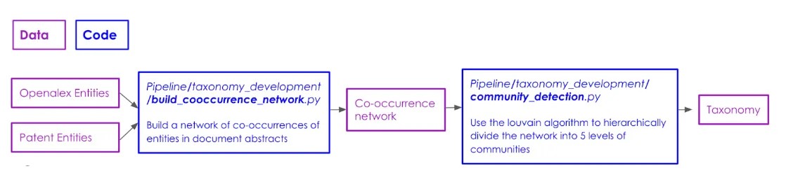
The first step in this algorithm is to generate the network of entities. Each node in the network is a unique Wikipedia entity extracted from the abstracts of patents and publications. The weight of a node represents the count of occurrences of each entity across both sources of text.  In order to reduce noise, we exclude all nodes with weight < 10. If two entities appear together in the same abstract, we connect them with an edge. Edge weights represent the association strength between the nodes. 

               

The second step is to build the taxonomy using the Louvain method for community detection. We force the taxonomy to be hierarchical by recursively splitting the network with increased resolution at each step. The algorithm starts at step 0 by splitting the network described above with a resolution of r = 1 into communities.  At each subsequent step i : {i = 1,...,4}, we generate subgraphs of the original network using the communities generated at the previous step. We then split the subgraphs containing at least 10 nodes into communities with resolution ri = ri-1 + 1. The algorithm continues recursively for 4 steps. The starting resolution and resolution increments are tuned to generate the most evenly distributed community sizes at each step using metrics described below.

Clustering of semantic embeddings

A potential concern with building a taxonomy from entity co-occurrences is that some high-weight edges may reflect spurious relationships between words and not a meaningful thematic connection. In light of this, we explored the use of semantic embeddings as an alternative to the network of word co-occurrences. We experimented with two different approaches to building the taxonomy using the SPECTER vector representations of DBPedia entities (see this section of our Github repository to explore the code used to generate these taxonomies). 

The methods described here are a subset of all the approaches considered, which include one of many clustering algorithms, GMM-based overlapping clusters, and manifold group-and-rank clustering. Future work will seek to further iterate on some of these and bring together both semantic and network-based approaches, capturing both explicit context relations as well as implicit semantic connections.

Centroids Clustering

The first of the two main methods presented, centroids clustering, uses scikit-learn’s K-means clustering algorithm (check out the documentation to learn more about it) to create the first layer of the taxonomy by grouping together the vector representations of all individual DBPedia entities, irrespective of their corpus frequency. We tune the number of clusters at this level by maximising the silhouette score of the candidate clusters while maintaining a relatively consistent number of final clusters as were obtained from the networks approach. 

                                                                                                                                        

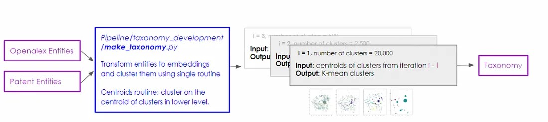
In the next step of the process, we identify the centroid of each resulting cluster. In a subsequent iteration of the algorithm, these centroids are used to form new clusters. The number of clusters set for each iteration is again chosen based on its ability to maximise the silhouette score.

Imbalanced clustering

The centroids clustering algorithm did create clear groupings of the DBpedia entities, but it proved unwieldy as it quickly created large components and concentrated large proportions of the entities on a handful of topics. In an attempt to lessen the chance of the taxonomy ending up with an exceedingly large main component, we developed an alternative method that bounds the average size of clusters in the taxonomy.

This second method also utilises scikit-learn’s K-means clustering algorithm, but it diverges from the first by constructing the taxonomy in a top-down manner. To initiate this process, we set the number of clusters to match the number of groups at the top level of the networks clustering approach, which creates a few clusters of many entities each. 

                                                                                                                                  

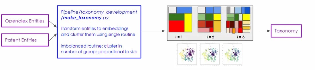
In subsequent steps, we apply the clustering routine on all individual groups defined in the previous (higher) level. However, the twist here is that the number of clusters is defined proportionally to the size of the input cluster, with a minimum threshold of 10 entities. In all scenarios, this approach gave rise to more finely divided clusters, although it was observed that this created uneven levels of granularity across levels in the taxonomy.

Validation

We experimented with various methods to create the taxonomy of academic and industry topics, but we needed a way to compare the results across methods and ensure accuracy and robustness. We developed a suite of metrics to evaluate different aspects of the taxonomy generated by each algorithm. The metrics were divided into three categories.

1. Distribution metrics: assess the distribution of DBPedia entities per group at each level of the taxonomy. 
2. Content metrics: assess the relatedness of entities grouped together at each level using human-defined topics.
3. Sensitivity metrics: assess the sensitivity of each algorithm to changes in the sample of entities included in the corpus.

 

Visit this section of our Github repository to explore all of the code for validation. The pipeline follows the below workflow:

                                                                                                                 

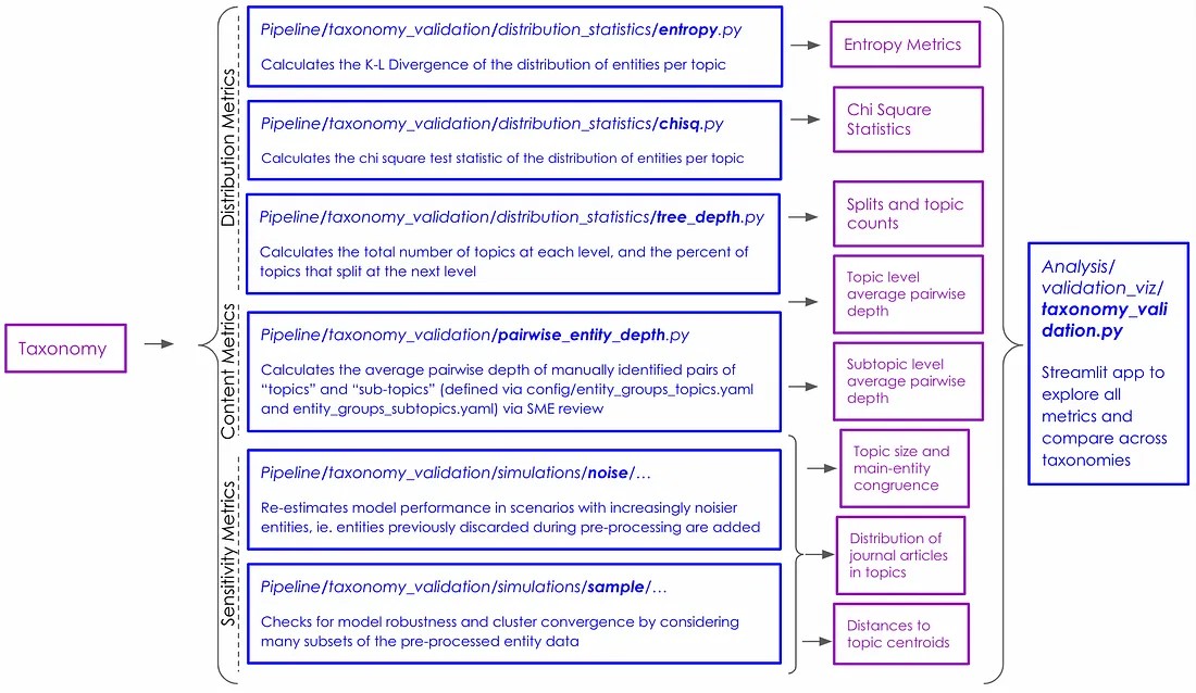
Distribution Metrics

We recognized that the landscape of research can rarely be perfectly partitioned into an even five-level hierarchy. For instance, certain disciplines might contain more areas and topics than others. Despite this, we needed a reasonably evenly distributed taxonomy for it to be practically useful. For example, if all “topics” were grouped together in the same “area”, measuring innovation across areas would be rendered meaningless.

We also sought to test how granular the splits were at each level, and determine how far into the five-level taxonomy each group continued to split, in order to ensure that the splits broadly resembled a natural structure of disciplines, domains, areas, topics and sub-topics.

The following metrics were used to evaluate the distribution of entities per topic – specifically evaluating if the distribution was even across topics, and how far into the taxonomy each topic continued to split.

1. Kullback-Leibler divergence:  this measures the relative entropy between the distribution of entities per topic (at each level) and a uniform distribution.
2. Chi-square test statistic: similarly to above, this tests the null hypothesis that the observed distribution follows a uniform distribution
3. Histograms: we also looked at histograms of the distribution, although this was not possible at deeper levels.
4. Split percentages: this calculates the percent of groups at level i that continue to split at level i+1. Because we implemented a stopping criterion of a minimum of 10 entities per group, many groups stopped splitting before reaching the bottom level.

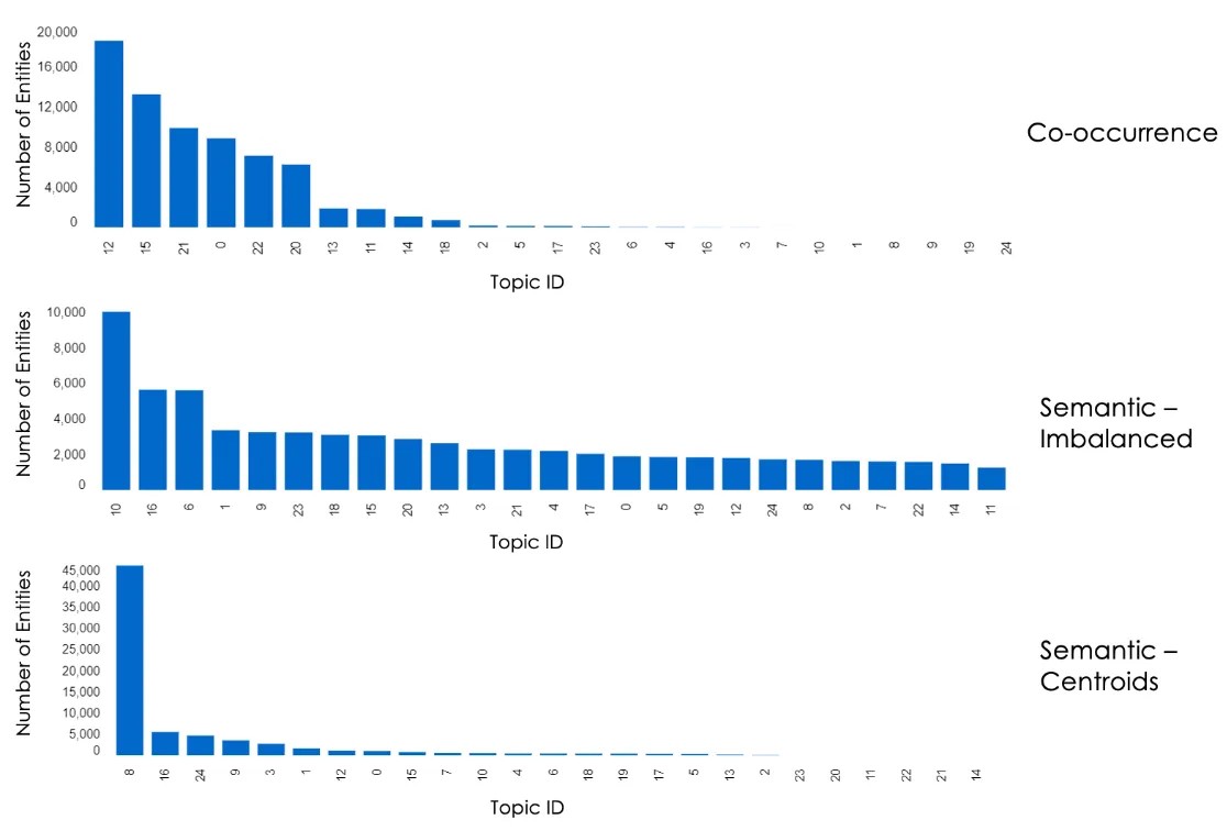
The figure below shows a histogram of the distribution of entities per discipline (top level of the taxonomy) using the various algorithms:

                                                                                                        

Content metrics

The suite of content metrics were designed to evaluate whether the taxonomy developed by each algorithm was in line with how experts in various fields would break down their domains. These metrics used both manual input from subject matter experts and comparisons with academic journals.   

• Subject Matter Expert Review

We generated two gold standards of DBPedia entities – one at the topic level and another at the subtopic level. These standards comprised entities (topic level and subtopic level) of Wikipedia Entities that experts believed should be grouped together.

1. Topic-level gold standard: this was generated using Wikipedia’s Outline of Academic Disciplines.
2. Subtopic level gold standard: this was generated by members of our team who have at least graduate level background in various disciplines. 

An example subtopic level breakdown is illustrated below:

natural_science:

  biology:

    neuroscience:

DBpedia tags: [Nervous system, Neuron, Computational neuroscience, Synapse, Axon, Neuroplasticity, Functional magnetic resonance imaging, Brain mapping, Diffusion MRI, Default mode network, Blood–brain barrier, Brain–computer interface]

We then calculated the Average Pairwise Depth at which any pair of related entities from the gold standards remained within the same group in our taxonomy. The depth here refers to the levels of the taxonomy.

• Journal similarity: 

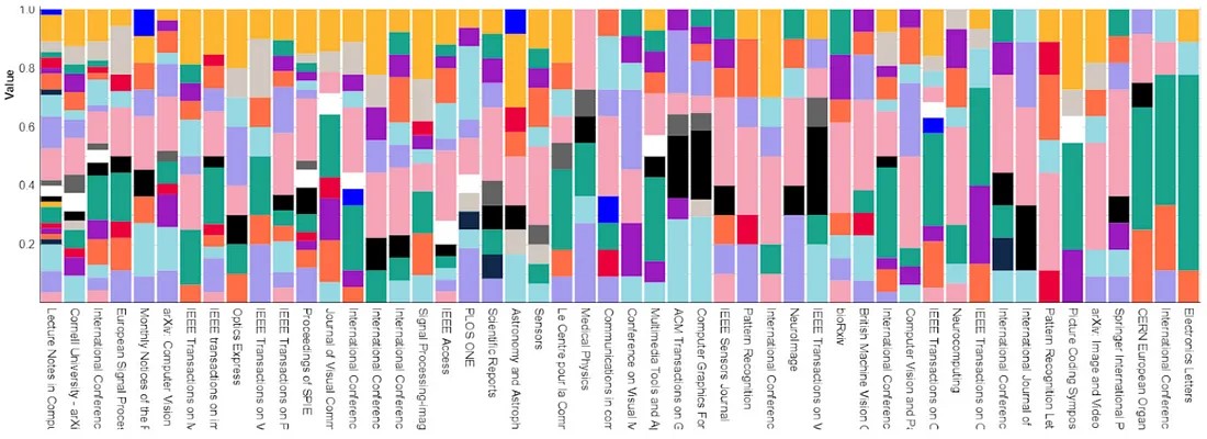
We also used Academic Journals as another type of “gold-standard”. We compared the concentration of topics within academic journals, indicated by the frequency of entities in their published articles, with the topic assignments to these entities. The expectation was that the distribution of entities would be highly correlated with the nature of the journal. For instance, cross-disciplinary journals would encompass a diverse range of topics, while field-specific journals would showcase a high concentration of a few topics directly related to the journal’s field.

The below graphic shows the distribution of topics from our taxonomy (indicated by size of each of the coloured bars) within a given journal.

                                                                                                    

Sensitivity metrics

We designed a series of experiments to measure (1) the sensitivity of each of the algorithms to different samples of entities; and (2) the sensitivity of each of the algorithms to the addition of noise (entities that had been previously discarded from the sample). These were meant to identify which algorithm would be the most resistant to small changes within fields, and therefore the most robust over time. 

For each set of experiments, we measured several metrics:

1. Relative topic sizes: used to test whether the introduction of noise or sample selection creates larger or smaller principal components, as well as the distribution of sizes as described in the above section about distribution metrics.
2. Distances to topic centroids: used to evaluate whether entities end up in more dispersed average topics when reducing the data size or adding noise.
3. Average pairwise depth of known pairs: given a pre-specified set of entities that field experts consider should be included within a given topic (as described above), we test the frequency with which this is true under different stress conditions.

Labelling

Each of the taxonomies described above were defined by different groupings of Wikipedia entities at various levels. However, we needed a method to create meaningful names for these groupings to present in our analysis. We experimented with several methods: entity labelling, journal labelling, and chatGPT labelling.

Entity labelling

This method named entity groups using the entities themselves. Entity groups were labelled using the five most common entities contained in the group. Commonness was defined using counts of the entities in all abstracts in the corpus.

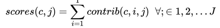
Journal labelling

This method labelled entity groups with the names of the most relevant academic journals to that group. 

We estimated the marginal contribution of journal j to group c via entity i as:  

                                                                                                                                 

Where 

• freq(c,i) is the frequency of entity i relative to other entities in group c
• freq(c,j) is the frequency of journal j in group c over other journals also present in c
• freq(j,ij )is the frequency of entity i in journal j relative to other entities in j

For each group c, scores for all journal contributions are then estimated as:

ChatGPT prompt engineering

This method provided ChatGPT (through the reverse API Python wrapper) with lists of entities in the group, and asked GPT 3.5 to name the cluster. Using this method, we were able to label the groups of entities, request confidence scores in the labels, and ask for entities that were considered “noisy” within the group. 

The prompts were as follows:

QUESTION: "What are the Wikipedia topics that best describe the following groups of entities (the number of times in parentheses corresponds to how often these entities are found in the topic, and should be taken into account when making a decision)?"

CLARIFICATION: "Please only provide the topic name that best describes the group of entities, and a confidence score between 0 and 100 on how sure you are about the answer. If confidence is not high, please provide a list of entities that, if discarded, would help identify a topic. The structure of the answer should be a list of tuples of four elements: [(list identifier, topic name, confidence score, list of entities to discard (None if there are none)), ... ]. For example:"

REQUEST: "Please avoid very general topic names (such as 'Science' or 'Technology') and return only the list of tuples with the answers using the structure above (it will be parsed by Python's ast literal_e method)."

EXAMPLE: "[('List 1', 'Machine learning', 100, ['Russian Spy', 'Collagen']), ('List 2', 'Cosmology', 90, ['Matrioska', 'Madrid'])]"

Pruning

The construction of a comprehensive and effective taxonomy is not complete without a nuanced pruning process, by which we refer to the act of selectively removing or adjusting elements in our taxonomy that do not serve the objective of clear categorisation. 

Firstly, we cleaned our named groups from the previous section using the lists of entities ChatGPT identifies as unrelated to other concepts in the group. ‘Back of the envelope’ validation using vector distances to group centroids confirmed that this is largely equivalent to thresholding a maximum distance of the entities’ vectors to the group’s average vector representation. 

A second step involved the extraction of location-specific entities. Using queries to GPT models, we identified entities that associate with countries and locations. These entities were then used to create new top-level topics in our taxonomy, dedicated to geographic locations. 

Following this data-driven pruning approach, we made a few additional manual adjustments to further refine our taxonomy, ensuring it effectively represented the landscape of research and innovation activities in the UK. This combination of automated and manual pruning helped us to ensure a coherent and meaningful taxonomy.

Conclusion

Using the methods described above, we decided to leverage the co-occurrence network taxonomy, labelled via ChatGPT, to conduct our analysis. There is no objective optimum taxonomy and we acknowledge limitations about using purely unsupervised methods. However, we made some decisions based on the desired qualities of the taxonomy for our use case. We found (through the methods described in Validation) that this algorithm produced a taxonomy that was reasonably distributed while still reflecting how experts divide the landscape of innovation. It was also the most resilient to the stress conditions described above. The ChatGPT labels were best at providing meaningful labels to people interpreting the analysis. 

This taxonomy served as the basis for an analysis of innovation across the UK, measuring things like novelty (check out this paper for more information on novelty) and disruption (check out this paper for more information on disruption) across disciplines, domains, areas, topics, and subtopics. 

Visit this Github repository for instructions to download the taxonomies and basic utility functions to assist in using them in your own code pipelines.